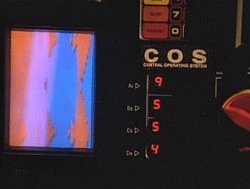
Jekyll2026-10-20T01:12:47+00:00https://vinurad.github.io/feed.xmlVinura Dhananjaya GalwadugeNotes and writeups on causal machine learning, large language models, and assorted technical work.Vinura Dhananjaya GalwadugeAI and Us-12026-10-18T00:00:00+00:002026-10-18T00:00:00+00:00https://vinurad.github.io/blog/misc-other/ai-wars-1I recently had the chance to watch an episode from X_Files, which shows an AI gone rogue (S1, E7, “Ghost in the machine”). The story shows an intelligent operating system becoming sentient, and taking actions for its survival. I do not remember how I felt when I watched this when I was younger (at least 10-15 years ago). The show itself was a favourite of mine, and somehwat inspiring too. But, this time, as I watched this with my wife, it was only a bit amusing to me. Nevertheless, we agreed that it must have felt very differently to the people back then. Did we find it only amusing because AI itself has become more familiar to us? Or is it that we downplay such scenarios involving AI? or is it because we already know that it is a possibility?
Only weeks ago, HuggingFace hack happened (https://metr.org/hugging-face-incident-report-aug-2026.pdf). Frequently, researchers state the risk of AI becoming rogue, and perhaps threatening humanity. Some argue that such threats are not credible and current AI is merely mechanistic and dumb. Especially, some argue that most of these (including other claims about present AI capabilities) are only marketing tactics, inflating the facts and perhaps nothing other than result the irresponsible practices of some AI companies (https://www.youtube.com/watch?v=54Lu6_ZRF0c). As I think, If we look beyond (or maybe not beyond, just nearby) this possible threatening nature if AI, we may see that AI poses a different kind of dilemma, which is our ‘dependency’ to it, which could be a very costly one.
I believe all these ideas have already been discussed or argued about, but here are my two cents. Throughout the history, many dilemmas that the humankind faced have been of our own making. Wars and their implications are obvious examples. Certain Non-commucable diseases (except for unfortunate causes such as genetics) are another example. The unprecedented implications of AI could be just another similar example in the future. One way it could happen is due to our dependencies on it. Currently, such dependency has been created, and being reinforced as the time goes by. As intellectuals argue this may or may not create other associated problems, such as a genration of people who do not think well (cognitive dependency), the resource consumption etc. Yet, it is really difficult to get away from the dependency as well. I think the primary reason is that the efficiency boost that AI is capable bringing into economic activities does not give an incentive to turn away from it. Only a bigger incentive such as preventing a risk to human safety/health would do otherwise. Another reason for dependency is that the values individuals attribute to certain AI systems (e.g., chatbots that are seemingly intelligent), as if they have intelligent capabilities. This masks possible blind spots that they obviously possess, and perhaps strengthen with the time, and more interactions. Perhaps, just as social media/short content cater to our boredom, and anxiety in a way (and thus woresening it with time), AI might be doing that in an unseen way.
Yet, as humans try to adopt AI in safety critical tasks (such as autonomous tasks that is already using AI) more and more, there may be better chances to realize and solve those problems. On the other hand, people do not learn lessons from their past mistakes (not true to every case, but surprisingly at some disastrous cases. e.g.- wars), especially when it involves attracitve incentives. The disruptiveness (or distructiveness) of some modern age decisions are only coming into light now (unfiltered digital media and short content). Should there be a major fault of AI that pose a visible threat to humans collectively, so that more eager guardrails would be applied, and make humans rethink about the dependency to AI? or would such a case still give power to a limited set of individuals? In a next post, I’d like to think about what long term implications, interventions should there be regarding AI adoption.
Update (19 Oct 2026): I did not that there was a paper presenting a mathematical model of LLMs as a cognitive virus (https://arxiv.org/pdf/2609.03344). I think this is a reference to what was mentioned earlier, where AI behaves in a similar way to Social media ( in terms of cognitive impediments).
This post is licensed under CC BY-NC-SA 4.0. The X-Files still is excluded and remains the property of its copyright holder.
Let us look at an example problem involving a causal influence diagram. The problem is about an oil widlcatter. I think that this is a popular use-case/scenario in decision sciences. The decision to drill is a high risk and a highly rewarding if successful. The problem has been studied previously in publications such as Shachter et al., 2013 (https://arxiv.org/pdf/1304.3108) and Raiffa 1968 (Decision Analysis: Introductory Lectures on Choices under Uncertainty).
Wildcatters are known as the popele who drills wildcat wells, which is a hugely risky venture but gives an advantage over others, if succeed.
The wildcatter must make a decision to drill (or not) a particular location for oil. There is a test result that provides some information about the presence of oil. However, the test result can be 10% wrong. There is also the chance that oil will not be there at all (60%). The cost of the test is 10 (xe6, USD. For ease, 10 units). If they drill, the reward of finding oil is 100 units, and the loss is -40 units if they do not find it. There is no reward for not drilling (except for the cost of the test that they decide to do the it and do nothing afterward).
The test can also be decided to taken or not (considering its cost). The decision to drill is based on the knowledge that the test was done or not (‘sufficient recall’).
Figure 2. Causal influence diagram of the oil wildcatter problem. Rectangles are decisions, circles are chance nodes, diamonds are utilities. Dashed arrows are information links.
The optimal decisions
Let us first calculate the expected utilities of drill/not drill for the scenario where they decide to do the test and it comes back as positive (oil present) (T=1, R=1).
In order to compar the expected utilitites, it is sufficient to compare only the joint probabilities of events. Because,
\(P(w \mid Pa(D))=P(w,Pa(D))/P(Pa(D))\). We would try to find the conditional probabilities of \(w\) (the unobserved world) given the available information for the decisions (\(Pa(D)\). Here, it would be the situation where we calculate the possibility of oil being actually present, based on the test results. When we compute these for each decision at our decision node (here, drill or not drill) the normalizing \(P(Pa(D))\) will be similar, which can be ignored for comparison. However, to calculate the actual utilites the normalizing step must be done.
Here, regardless of the decision, there is always the cost of the test (-10). We can also ignore it as it is common for every decision.
Comparing these unnormalized utilities, it seems that it is the best to trust the test result always.
]]>Vinura Dhananjaya GalwadugeNotes on causality in games2026-09-30T00:00:00+00:002026-09-30T00:00:00+00:00https://vinurad.github.io/blog/causality/Notes-on-causality-in-gamesIntroduction
The parts up until section 2.2 describes the problem and an introduction to Structural Causal Models (SCM) and Pearl’s hierarchy of causality.
MAIDs
An ID (Influence Diagram) generalizes a BN by introducing decision and utility variables. A MAID (Multi Agent ID) extends it to a scenario with multiple agents. At the core, this captures an EFG in a more compact way (the branches in EFG captured in the nodes and their associated CPDs). There are chance nodes, decision nodes and utility nodes. The decision nodes describe decisions (or actions) made by agents, either as deterministic rules or stochastic rules. A decision rule is denoted as a CPD (below),
\[\pi_D(D|Pa_D)\]
A Nash Equilibrium describes the best response decision rule of an agent to those of other agents, and the parameters of the game (chance variables).
s-relevance and s-reacheabiliy
s=strategically. s-relevance tells if a particular decision rule impact another decision rule, i.e- changing one gives incentive to change the other or strategically relevant. s-reacheability tests if a
This has a similar notion to d-connectedness in causal graphs.
Mechanized MAIDs
Call $V$ the variables (nodes) in MAIDs. Mechanized MAIDS (MMAIDs) add a new variable set $M$, and $m_v in M$ are parents of each $v \in V$ (where necessary).
Each $m_v$ is either a decision rule variable $\Pi_D$ or a parameter variable $\Theta_V$.
A mechanized graph $\mathcal mG$ is simply the MAID plus $m_v$ and extra edges from $M_V \to V$ and edges within $m_v$ ($E’$, not self loops, but may have cycles).
The decision rule variables are policies that determine the actions (decisions) at the decision nodes (or the probability distribution of them). For example, a policy tells to always take a particular decision if some condition is met.
\[P(d|pa_D,\Pi_D=\pi_D)=\pi_D(d|pa_D)\]
With this addition, we can intervene over the CPDs of the decision variables, unlike the given CPDs in MAIDs.
The mechanisms that sets utilities and the chance are parameters; $dom(U) \in \mathbb R$.
The addition of new variables now allow to model the changes of an agent’s policy (how they pick decisions) and the impact of those changes to other agent’s policies. For example, $\Pi_D=\hat\pi_D$ can be a certain rule, where the agent ‘always go regardless of their laziness’ (the example EFG describes the chance variable parameterizing lazy/hardworking).
Independent MMAIDs
Denoted by $\mathcal m \perp G$, removes all $E’$ edges. Mechanisms are independent (i.e. similar to non-requisite variables in BN).
Strategic play in games break this independence. Because in reality agents respond to the changes in mechanisms.
Rationality relation
Described as a function $r_D(pa_{\Pi_D})$, describes the set of acceptable decision rules $\pi_D$
R-rational response and outcome
R-rational response is any $\pi_D \in r_D(pa_{\Pi_D})$. R-rational outcome describes a profile $\pi$, in which every $\pi_D$ is the rational response.
PyCID Examples
The repository https://github.com/causalincentives/pycid has implemented the MMAIDs and contains a few examples.
]]>Vinura Dhananjaya GalwadugeConnections Of Ope To Causal Theory2026-09-13T00:00:00+00:002026-09-13T00:00:00+00:00https://vinurad.github.io/blog/Connections-of-OPE-to-Causal-TheoryVinura Dhananjaya GalwadugeIdentifiability of Causes2026-09-12T00:00:00+00:002026-09-12T00:00:00+00:00https://vinurad.github.io/blog/causality/Identifiability-of-CausesIntroduction
This was written based on one of the exercises (problem 3.8) from the book “Elements of Causal Inference: Foundations and Learning Algorithms” by Jonas Peters, Dominik Janzing and Bernhard Scholkopf, which is a great read on the foundations of causal theory. The problem descirbes two random variables that can belong to one of two possible Structural Causal Models (SCM).
\[\begin{aligned}
X &:= Y + N_X \\
Y &:= N_Y
\end{aligned}
\qquad \text{(SCM 1)}\]
or,
\[\begin{aligned}
X &:= M_X \\
Y &:= X + M_Y
\end{aligned}
\qquad \text{(SCM 2)}\]
In each SCM, the parent and the child are different (the cause and the effect are reversed). Also, both SCMs have the exogeneous noise variables ($N_X, N_Y, M_X, M_Y$) following different Gaussian distributions (i.e.- different means and variances that are non zero). The problem is if we can identify which is the cause and effect, only using interventions. We do not know the nature of the noise distributions at all (i.e.- the parameter values are unknown).
To quickly state what an intervention is; we intervene on a desired random variable by changing its value. Theoretically, there are two main ways how this can be done (hard, soft). Here, hard interventions (directly setting a random variable to a specific, known value) matter.
Solution
Below is one possible real world example.
Suppose there are two electric light globes, which is connected to each other through some unknown circuitry. Their light intensity appears to be random, and we can measure it. Unknown to us, one globe’s light intensity controls the other (we do not know which controls which). We only know that the control mechansim could be either one of the above SCMs. Also, we can manually set the intensity of a globe to a fixed value (an intervention). We cannot know (even my measuring) their original distributions, and only measure after an intervention. The goal is to find which one is the unknown mechansim. Note that, this example forces the mean values of the distributions to be positive as the light intensity must be some positive (or zero) value, but I believe the example works fine.
First, we shall set the intensity of Y to 2 (i.e.- \(\mathrm{do}(Y=2)\), and the units are measured with some standard intensity unit). We would then measure the light intensity of X by taking many samples. If the mechanism follows SCM 1, X would show a different distribution than its original (unintervened on Y) distribution. If it follows SCM 2, then X will not change its original distribution. Unfortunately, we cannot still distinguish between the two scenarios as we do not have any knowledge what those different distributions should look like, as we do not know their original distributions.
\[\begin{aligned}
Y &:= 2 \\
X &:= 2 + N_X
\end{aligned}
\qquad \text{(SCM 1)}\]
\[\begin{aligned}
X &:= M_X \\
Y &:= 2
\end{aligned}
\qquad \text{(SCM 2)}\]
In each of the above equations, the non-intervened variable $X$ still follows a normal distribution (mean shifted), which cannot be distinguished from each other as we do not know the original distribution parameters.
Now, let’s do another intervention (\(\mathrm{do}(Y=3)\)). This time however, we can observe and measure a difference. In SCM 2, $X$ will still follow its original distribution, while SCM 1 will show a mean shift from the previous intervened distribution.
This is similar to an increase in the average light intensity in our example. Practically, this second intervention could be done as a drastic change of the value, so that the change is visible to the eye.
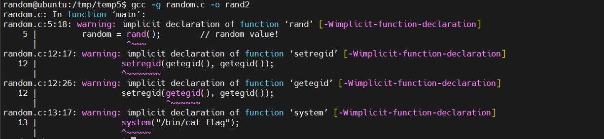
]]>Vinura Dhananjaya GalwadugeVllm On Hpc2026-09-07T00:00:00+00:002026-09-07T00:00:00+00:00https://vinurad.github.io/blog/vLLM-on-HPCVinura Dhananjaya Galwadugepwnable.kr - random2026-02-15T00:00:00+00:002026-02-15T00:00:00+00:00https://vinurad.github.io/blog/misc-tech/pwnable-randomThis is the 4th challenge in ‘Tolddler’s Bottle’ in pwnable.kr. The ‘rand()’ function is supposed to generate pseudo-random numbers when a seed is given. The thing with psuedo-random number generators (PRNG, such as rand()) is that they provide deterministic outputs for a given seed. Usually, ‘stdlib.h’ is required to properly declare rand(). The given code does not contain it - hence a compiler warning is raised.
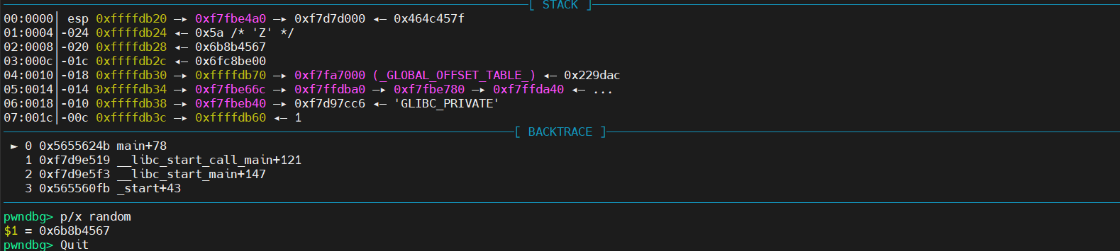
Then how does rand() work? If the linker can correctly match it during the runtime, rand() runs. In fact since the implicit assumption of a function call matches rand() implementation (the output is int and the function call is rand(void)), it runs. However, in the process, the seed does not change. The results is the random value is the same each time (not random!). This value can be obtained as below.
The goal is to uncover the flag by using the correct key. In this case,
\(\mathrm{key} \oplus \mathrm{random} = \mathtt{0xcafebabe}\)
\(\mathrm{key} = \mathtt{0xcafebabe} \oplus \mathrm{random}\)
This is because, XOR operation’s identity property (XOR’ing the same variable is just unit). The returned value is 0xa175ffd9. We are supposed to provide a decimal as the input to the program. However, a caveat is that although the key is initially declared as an ‘unsigned int’, the ‘scanf’ reads the input as a ‘signed int’ (‘%d’). The decimal of the previous 0xa175ffd9 is 2708864985. This is larger than the max. positive for 32-bit signed integers. If we use an online tool like ‘rapidtables’(https://www.rapidtables.com/convert/number/hex-to-decimal.html), it shows the 2’s complement of an input value as well. In this case, the 2’s complement of 2708864985 is -1586102311. The ‘scanf’ function would store the value corresponding to the 2’s complement of -1586102311, if we give it as the input to the program. Also, this value is in range of the 32 bit signed ints.
This reminds me of something one of my instructors said; “The bits do not have any inherent meaning, but the meaning we give them”. Giving this negative value as the input to the program will reveal the flag.
The Hodge-Laplacian (HL) operator is a generalization of the node (graph) Laplacian operator. Below are some key ideas related to the HL operator.
Simplices
Simplices are the structural building blocks of a graph. A 0-dimensional simplex is a node, and a 1-dimensional simplex is an edge connecting two nodes.
Boundary operators on a graph
Boundary operators take two simplices as the inputs, and represent a relationship between those two simplices (e.g., a node and an edge). Let us denote boundary operators by $B_k$. Here, $k=1$ would mean that it would take a max dimension of 1 for one of the input simplices (an edge). The other would be 0 dimensional (a node). The $B_1$ operator on vertex $i$ and an edge $e$ would look like below,
\[(B_1)_{i,e} =
\begin{cases}
1 & \text{if } i \text{ is the tail of edge } e \\
-1 & \text{if } i \text{ is the head of edge } e \\
0 & \text{otherwise}
\end{cases}\]
Applying a boundary operator on a node signal (feature) would return
Graph Laplacians
Graph Laplacian or node Laplacian (unnormalized) ($L$) is known as $L=D-A$. $L$ is taken as the difference of the degree matrix $D$ and the adjacency matrix $A$. It can also be observed that $L=B_1B_1^T$. The graph Laplacian operator can be understood as an operator that filters (specifically, a low-pass filter) that operates on the node level, and smooth the node level signals (representations) throughout the graph.
Hodge Laplacian
Hodge Laplacian is a ‘higher-order generalization’ of graph laplcian [1]. While the node Laplacian operates at the node level, the Hodge Laplacian operates at edge level and beyond.
HL operator
HL operator is also a type of Laplacian operator. It is formally defined as $\mathcal{L}k=B{k+1}B_{k+1}^T+B_k^TB_k$. When $k=0$, $\mathcal{L_0}$ becomes the node Laplacian operator that operates on node signals. When $k=1$, HL becomes an operator at edge level and the triangle (2-dimensional simplices) level. While the node Laplacian operates on node signals (or nodes), the HL operator works at higher levels structures such as edges, or triangles and their signals. In other words, HL operators can act on more complex graph structural relationships (in general) such as node-edge, edge-edge or edge-triangle relationships while the node Laplacian is limited to node-node level.
References
[1] - Hodge Laplacians on Graphs, Lek-Heng Lim, https://www.stat.uchicago.edu/~lekheng/work/psapm.pdf