Introduction

The main goal of this article is to provide a high-level intuition of market making (MM), its goals, and the Avellaneda-Stoikov algorithm for MM. I believe the structure of this article aligns with how I came to understand MM and the surrounding concepts and it does not follow any formal structure.

Preamble

To start with, think of traders whose main goal is to make profits. There are many ways to do this.

Keep a stock (an inventory) of some assets (e.g., gold) and hope to gain some profits later by selling them (“long”).
Traders can lend their assets (e.g., gold) and make some money out of it. … k. Traders do not plan to keep an inventory of assets. They’d rather buy them for a low amount and sell them for a higher amount, repeatedly.

In the MM context, it is the kth category that is of focus. Traders of this nature consider keeping an inventory risky. A number of good examples can be found in the crypto market. People keep inventories of coins to find their value crash later. Instead, it is preferred to do quick (or high frequency) trades of buy-low, sell-high nature and make profits.

The dynamic nature of markets

Modern stock markets, crypto markets (or broadly, securities markets) are excessively dynamic in nature. Their order books (or Limit Order Books - LOBs) move at high frequency, which requires a similar pace in placing a trader’s buy-sell orders.

A simple strategy

A trader would buy securities some amount below the mid price in the LOB (bid price), and sell at some amount above the mid price (ask price). Determining these two prices would determine the amount of profits. A naive strategy would be to set these prices by subtracting or adding a fixed amount to the mid price.

\[P_a = s_t + \delta\] \[P_b = s_t - \delta\]

Avellaneda and Stoikov algorithm

The paper by Avellaneda and Stoikov shows a better strategy than the simple strategy. Well, how is it better? This algorithm (let’s call AS) aims to control the inventory - hence it can control the risk. Before that, let us look at how having an inventory can pose risk. This is also called “inventory risk”.

Inventory risk

Example 1: The trader holds the assets (long) and never sell and the mid price goes down. Now the asset loses its value.
Example 2: The trader does not hold all the assets, but keeps a little amount (let’s say they keep 50% and sell the rest). Still, if the mid price goes down, the asset loses its value and it may overpower the profits gained ($P\&L < 0$).

There may be instances that holding the asset would yield better gains in the future. But that is not the focus of the trader’s strategy we discussed in the preamble.

Another related term is “transaction risks”. When the trader has posted both buy and sell orders, there is a chance that incoming orders may fulfill only one of them (or one type) for a long period.
If only buy orders are filled - inventory risk
If only sell orders are filled - the trader may lose profit (do not have enough inventory to keep the trade going on).

We can see a pitfall of the simple strategy here. As it is not sensitive to the state of the inventory, it is prone to inventory risk. (i.e., we may keep filling our bids or buy orders).

AS provides workarounds for this. The main derivations from the paper are:

\[r = s_t - \beta q\] \[p_b = r + \delta^*\] \[p_a = r - \delta^*\]

The amount $2\delta^$ is called the optimal spread. Before stating how $\beta$ and $\delta^$ are calculated, it is of our interest to know what they do. $q$ represents the current inventory (or the number of assets the trader has). The main objective is to control $q$ close to $0$ as much as possible. Hence, $r$ would be greater than $s$ (the mid price) if we have $q < 0$. This means we are inclined to buy a bit higher than the mid price (increases our buying chances). If it’s $q > 0$, we are trying to sell a bit lower than $s_t$ (increases our selling chances).

However, this alone will not yield profits (we are buying high and selling low). Hence, we make adjustments to our $r$ by $\delta^*$ amounts, which gives us optimal ask and bid prices.

Another key intuition to have is that the higher the $\delta^*$ is, the higher the chance that the orders do not get filled. This comes from the fact that the majority of the other orders would be closer to the mid price.

From the paper:

\[\beta = \gamma \sigma^2 (T - t)\] \[\delta^* = \frac{1}{2} \gamma \sigma^2 (T - t) + \frac{1}{\gamma} \ln\left(1 + \frac{\gamma}{k}\right)\]

$\gamma$ is the risk aversion degree (inventory risk) set by the trader. The higher the value, the more risk averse. $\gamma_{min} = 0$ which is risk neutral. $\sigma$ denotes the volatility of the asset. $T$ and $t$ denote the end time (the trader trades) and the current time, respectively. $k$ is the liquidity parameter of the LOB. This measures the intensity of the arrival of orders that can fill the trader’s bids and asks. If the $k$ value is high, then there is a higher chance that the order does not get filled if $\delta^*$ is also high.

Key high level takeaways from the formulae

The reservation price ($r$) makes an adjustment to the mid price, toward the direction opposite to the current inventory state.
With this, $r$ makes sure that the inventory is close to 0.
At the beginning of the trade ($t=0$), this adjustment is the highest. As $t \to T$, the adjustment becomes weaker, making $r$ closer to $s_T$. This makes the limit orders toward the end almost like market orders, ensuring that they get fulfilled and no inventory would be left at the end.
If an inventory risk arises in the middle of the process, $r$ makes sure that the assets are prone to liquidation (more selling and less buying).
If more sell orders are fulfilled, then $r$ does the opposite of 4 by trying to buy more assets and making resistance to sell.
The more the volatility of the asset, the more the spread. It is similar to expecting more compensation for longing/shorting a volatile asset.

Results from the paper

The numerical simulations from the paper show the advantage of the algorithm in controlling the risk by controlling the inventory. This is evident from the lower standard deviation of P&L with the AS algorithm than the simple strategy. In other words, the simple strategy may give very high profits or very high losses.

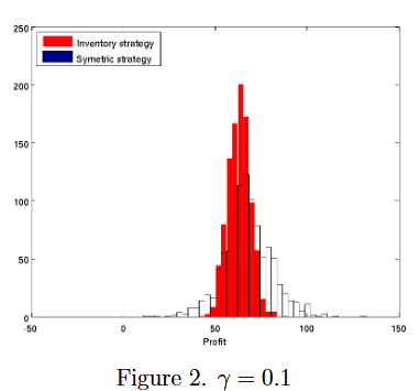
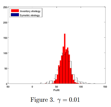
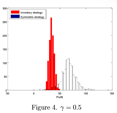
Figure from Avallaneda, Marco and Stoikov, Sasha, 2008.

The role of $\gamma$ is important as well. As $\gamma \to 0$, AS gradually becomes similar to the simple strategy.

References

High-frequency trading in a limit order book, Avallaneda, Marco and Stoikov, Sasha, 2008. (http://www.tandfonline.com/doi/abs/10.1080/14697680701381228)